All in One View
Content from Acquiring Raster Data using Imagery databases
Last updated on 2025-08-14 | Edit this page
Overview
Questions
- Where can I access raster and satellite imagery datasets?
- How do I download and use CORONA and Sentinel Imagery?
- What tools and platforms are commonly used for data collection in the field?
Objectives
- Learn how to download prescanned maps from public and academic websites
- Learn how to acquire historic satellite imagery
Introduction
Hard copies of maps, air photos, and other hardcopy images scanned at a high resolution are often georeferenced to provide useful context for other data layers in a GIS. Details of these raster background layers can also be digitized into separate vector layers for further analysis.
Beginner - Downloading Pre-scanned Maps
Several public and academic websites provide raster data, such as scanned historic maps, aerial and satellite images, and other media available to download at no cost. Scanned paper maps are usually downloaded as spatially “unintelligent” images, meaning they are simply scanned media that need to be georeferenced prior to use in a GIS. Other raster sources, such as imagery collected by modern satellites are already georeferenced. Additional sources of raster data are made available as direct-use services without downloading the data at all. Below, we provide some common raster data sources of different types. Explore them on your own to get a sense of the types of media they offer; the “About” page for each source is often a good place to start. In the next module, we’ll examine the search and download features in a few of these sources in more detail.
In the following modules you will locate and download examples of historical maps and satellite imagery (i.e., raster data) prior to using them in QGIS. (If needed, review the section on Georeferencing and Digitizing Points on raster images in the Data Management module.)
Download Historical Maps
Several websites offer scanned maps, but the repository we’ll focus on for this tutorial is the University of Texas Perry-Castañeda Library (PCL) Map Collection, which hosts thousands of scanned paper maps available for free download. The maps are organized geographically by region and country. In your web browser go to: https://legacy.lib.utexas.edu/maps/
- Scroll down and click on Historical
- Browse the topics until you find a useful map (feel free to browse the other geographic headings as well). Sometimes large map series, like military topographic maps, will have index maps that can help you find a specific area of interest
- To save a map, right click on it and select Save Image As and save it in your project folder. Follow a similar process to explore and download scanned maps form the other sources listed above.
Intermediate - Acquiring satellite imagery
Another important source of historic raster imagery is from declassified spy satellite imagery developed in the mid-20th century. In this tutorial, we will learn to search for historic satellite imagery on the CAST and USGS websites, which require a few more steps than downloading a scanned map. With advances in orbital space flight during the Cold War, the US developed a series of classified space-borne optical imaging satellites for intelligence gathering purposes. The CORONA program (1960-1972) was the United States’ earliest photo reconnaissance satellite program producing over 860,000 black-and-white images, comprising the first high-resolution (up to ~2m) stereo images of the earth’s surface. The images were declassified by the Clinton administration in 1995. The highest resolution CORONA images, produced by the KH-4B series of satellites between 1967 and 1972, were collected by a panoramic camera on long, narrow film strips, each covering a land area of about 8.6 × 117 km. High-resolution scans of original CORONA negatives are available to download from the USGS EarthExplorer website for free at a maximum resolution of 3600 dpi (7 microns), or for $30 per frame for scenes that require a new scan. Since they became available to the public, CORONA images have played an important role in the study of historic landscapes to identify archaeological sites, old land tenure systems, and landscape features now obscured or destroyed in recent decades by industrialization, urban expansion, and agricultural intensification.
Search Georectified CORONA imagery on CAST website
In many cases, CORONA imagery requires georeferencing to be used in a GIS. However, some georeferenced Corona imagery is already available to view and download on the CORONA Atlas and Referencing System, an interactive web map at the University of Arkansas’ Center for Advanced Spatial Technologies (CAST) for downloading previously georeferenced scenes free of charge. This Beginner level tutorial will show you where to find it, and in the Intermediate level tutorial that follows you will search for a wider database of imagery on the USGS EarthExplorer site that will require georeferencing. While not all the Corona imagery available elsewhere is on it, it is nevertheless a good first place to look for Corona images in your area of interest.
- In your web browser go to https://corona.cast.uark.edu/
- Click Explore Atlas
The red rectangles show the different Corona missions that were carried out and that are available to view and download on the CAST website.
- In order to view the available imagery, zoom in to one of these red boxes
- You can use the slider tool at the bottom of the screen to view CORONA and modern satellite imagery side by side
- You can move the slider next Corona Imagery to make it partially transparent
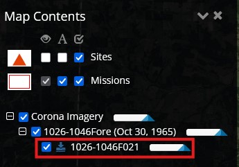
- Expand the Corona Imagery layer by presing the (+) button to see the details of the different images being displayed
It is from this list of Corona Imagery that we can download imagery from the site
- Zoom close into your area of interest
You will notice the number of visible CORONA missions listed will decrease as you zoom in.
- Expand each of the missions by pressing the (+) button next to them
- Turn off each image in turn in order to decide which is the one you want to download, and then click the blue dowload button (V) next to it
- Click Download GeoTiff, this will start the download - it is a big file so it will take some time
- Once it has completed, move the image from the Downloads folder to a new folder (e.g. CORONA) in your GIS folder
- Open QGIS and click the Open Data Source Manager button on the toolbar
- Click the Raster tab, click the browse button and find your CORONA image
- Click on it, then Open, Add and Close
Challenge
Download a Corona image in your area of interest, or of a famous landmark, from the CAST website.
Searching and Download raw CORONA imagery from USGS EarthExplorer
While the CAST website is a convenient first place to look for CORONA imagery, you may not find coverage in your area of interest. Since large areas are not covered in the CAST catalog, we are going to search for Corona imagery from the USGS EarthExplorer website which hosts the complete collection of CORONA imagery. The interface of EarthExplorer is not very user friendly which can make finding the right CORONA scenes a bit challenging, so this tutorial will assist you in locating the best available imagery for your study area.
- Begin by logging in or creating a free login account at the USGS EarthExplorer website: https://earthexplorer.usgs.gov/
- After logging in, the interface screen will have a map navigator on the right and a space for entering imagery search parameters on the left.
- In the map window, navigate to your area of interest. Use the mouse to click the corners of a polygon to define the area you’d like to search for imagery. Alternatively, zoom to your area of interest, and hit the Use Map button in the search Criteria pane. In both cases, your search interest will appear as a semi-transparent red polygon.
- Under the Data Sets tab, select Declassified Data > Declass 1 (1996).
- Select the Additional Criteria tab, then expand Camera Resolution and select Stereo High. This will limit the search to only the high quality KH-4B imagery.
- Optionally, expand Download Availability and select Yes to only show images that have been scanned and downloadable. (Some of the CORONA negatives are not yet scanned, but can be ordered for the price of $30. Leave this field blank to show the complete coverage.)
- Run the search by pressing the Results button, which will open the final “Results” tab.
- In the list of available images in the Data Set pane, use the “Footprint” and “Image Overlay” icons for some of the images to explore your results. To see all of the footprints at once, expand the Show Browse/Footprint Controls button and check Show All Footprints from Current Page.
- Next, for one of the images listed click the Show Metadata and Browse button (hint: hover your mouse over the center icon resembling a sheet of paper) to find out more about a particular image, such as its Mission Number; in the pop-up metadata window, click on the image preview to see it in greater detail. This is a good way to preview the image for cloud cover and clarity.
- Once you have decided on an image to download, click on the Download Options button (the hard disk icon with the green down arrow) and select Download. These are large files so they may take time to download.
Having downloaded our Corona imagery, you will need to unzip the folder and examine the files. This will also prepare for the later step of georeferencing the images in QGIS, or other GIS software.
- Navigate to your downloaded .tzg file and move it to your project folder
- Right click it and select 7-Zip > Extract Here
- Right click the new .tar file and select 7-Zip > Extract Here This will produce four new .tif files: the original image that has been split into four separate files ending in a, b, c and d.
Acquiring Sentinel-2 multispectral satellite imagery
The Sentinel-2 satellite program was launched in 2015 for the purposes of land-cover map production, soils and forestry research, disaster relief management, and other land surface monitoring goals as part of the European Union (EU) and European Space Agency’s (ESA) Copernicus Earth observation program (https://www.copernicus.eu/en). Since then, the twin Sentinel-2 satellites (2A and 2B) have provided the earth science and heritage communities with high-resolution, multispectral optical imagery across 13 spectral bands with a short revisit rate of about 5 days (referring to the period between passes over a site). Prior to Sentinel, the highest-resolution true-color imagery available to the public was 15m Landsat-8 data, so the sharper 10m Sentinel data offers a remarkable improvement. Sentinel imagery has been slower to catch on with some science communities due to its lower spatial resolution relative to commercial imagery (some of which available for free on Google Earth). Nevertheless, despite having a lower spatial resolution than commercial imagery, the high spectral resolution (in the form of multiple band combinations) and high temporal resolution (meaning rapid return rates) of Sentinel-2 imagery carries high potential value for social science studies of land cover analysis, human-environmental interaction, and heritage landscape monitoring applications. This tutorial will introduce you to the ESA Copernicus portal interface and guide you through the steps of searching and downloading Sentinel-2 imagery.
Navigating Sentinel Imagery from the European Space Agency Copernicus Browser website
- To gain free access to the ESA’s Sentinel data, begin by logging in or creating a free login account using the Register button on the Copernicus homepage: https://identity.dataspace.copernicus.eu/.
- You will then be redirected to the Copernicus Browser page (or navigate to it with this link: https://browser.dataspace.copernicus.eu/)
- Customize the language settings using the pull-down menu near the top-left corner of the screen.
- Use your mouse in the map pane to navigate and zoom to an area of interest
Downloading Sentinel Imagery from the European Space Agency Copernicus Browser website
- If necessary, log back into the Copernicus Browser page (https://browser.dataspace.copernicus.eu/)
- In the left pane, there are two tabs (Visualize and Search) with tools that allow you to filter and preview your Sentinel images in different ways prior to downloading them.
- With the Visualize tab activated, you can adjust
the following criteria to search from (starting at the top and moving
down):
- select the date or date range of imagery needed (or simply click “show latest data”). Days for which imagery is available in your area of interest are highlighted with a blue box.
- limit acceptable cloud cover with the slider bar (e.g., 10%)
- specify which Sentinel satellite you want data from (e.g., Sentinel-2, which will be the most useful for us here)
- in the “layers” section, select from several popular band combinations available for download (e.g., true color, NDVI, land cover classes, etc.)
- With your preferred criteria defined, click the Find products for current view link. This opens the Search tab and shows the specific scenes available in your AOI that meet your criteria and available for download. Each Sentinel scene listed in the Search pane corresponds to a green square in the map pane that is highlighted when you hover the mouse over the listed scenes. Detailed Information about each scene is available by clicking the i button for each listed scene, or selecting a green square on the map.
- The crosshairs icon for each listed scene will also zoom to that scene on the map.
- You can explore a scene further by clicking the Visualize button below a scene’s thumbnail image, which opens it in the Visualize tab, allowing you to explore the different band combinations.
- To change the date range, or refine the months in your search (e.g., to remove snowy winter months), return to the Search pane, click Go to search at the top of the pane, adjust your criteria as needed and click Search again.
To download an image, simply select the Download button on the right side of its listing. The size of the image is listed above the Download button, so it may take time depending on your connection speed. When it has finished downloading, you will find a SAFE.ZIP file in your specified folder, which can be extracted and imported to a GIS software for further visualization.
placeholder
Content from Basics of Feature Class Manipulation
Last updated on 2025-07-25 | Edit this page
Overview
Questions
- What are the three basic Vector data geometries?
- How do you create a feature dataset in QGIS?
- How do you decide what datapoints should be included in a dataset?
Objectives
- Understand the basic components of vector geometry
- Learn to create a data dictionary
- Learn the basics of data collection
- Learn to prepare a project file in QGIS
Beginner - Characteristics of geospatial data
Intermediate - Design and create a new feature dataset in QGIS
In this section, we outline the steps for creating a basic data collection workflow that can be accessed and used by students, collaborators, or public participants to collect field data on a desktop GIS or on a mobile device. The following steps assume that you have downloaded and installed a GIS software package (e.g., QGIS) and you have a new project open.
Design a layer to contain your incoming data
This is the most fundamental part of geodatabase design, and the most time consuming. This stage is where you will conceptualize what kind of vector data you need to collect to answer your research question, and how that translates into the spatial geometries of a GIS (e.g., points, lines, polygons, or all three).
First, consider what objects or phenomena field collectors will be recording to the map, that you will want in your database to later query, analyze and display for your project. Make a list of each kind of object or phenomenon you are interested in (e.g., variables in your study), since each may require a different data layer.
Think about what shape/geometry those objects and data points will be most appropriately represented as at the scale you anticipate analyzing and displaying them. (TIP: a building might best be represented as a point on a small scale map, but as a polygon on a larger scale map).
Next, brainstorm what kind of information (or, attributes) is important to collect about each feature in your layer. It can be helpful to use graph paper, spreadsheet software, whiteboard, etc., to create a table listing the kinds of information you want to collect, correlated with variables, measurements, or units, that can describe that information collectable as data. These will be driven by the variable your research is studying, so it is worth taking the time to map out these variables in a table format before creating your GIS layers. As an example, if you studying declining butterfly populations, the types of information that might inform your study could include information organized in the following table:
| Type of useful information | Example data points (attributes) |
|---|---|
| Traits about the butterfly | species, stage of development, condition |
| What time of day was it spotted? | date and time |
| What was the weather like? | temperature, cloud cover, precipitation |
| Was the butterfly spotted on vegetation? | plant species |
| What was the location? | park name, address, coordinates |
| Should collectors provide a general description? | description, comments field |
| Will a photograph be helpful? | field photo from phone |
-
Once you have brainstormed the categories of traits or attributes to collect about a feature or place, it’s time to translate these categories of data into spatial data “fields” that will form the attribute table for your GIS feature layer. This process can be referred to as building a “data dictionary”. Things to consider here: will each data point need a unique name or identifier code; will field collectors need to add measurements (if so, how precise); what kinds of observations will be entered in the collection form (numerical, textual, etc.); would pull-down menus be helpful to predefine selections available to collectors, should photos or attachments be added during data collection?
- Some data properties can be changed later as your project evolves, but some are more difficult to change once they are established. So here again, visualizing your data dictionary in a spreadsheet is helpful, as in the example below:
| Attribute Description | Field Name | Data type | Length (text) | Data entry method | Allow null values | Allow attachments |
|---|---|---|---|---|---|---|
| Butterfly species | Species | String | 40 | pull-down menu | no | yes |
| Time of day | Date_time | Date | Choose from calendar | no | no | |
| Location of sighting | Location | String | 40 | Enter text | yes | no |
| Vegetation host | Vegetation | string | 20 | Enter text | yes |
Prepare a project file and editable data layers in QGIS
- Make sure you have downloaded and installed the latest version of QGIS
- Launch QGIS and create a new Project using the blank page icon on the top right of the screen. Use the Save as… command in the Project tab to save your new project in a convenient location.
- To create a new feature layer, from the Layer tab,
select Create layer, then select New Shapefile
Layer. We can now configure the new layer properties:
- In the New Shapefile Layer window, set the File name of the new shapefile in the file path to “Butterflies.shp”
- For Geometry, select Point.
- Use the default coordinate system, e.g., WGS84.
- In the New Field section, we will create attribute fields based on the spreadsheet you made earlier in the exercise.
- Configure the data collection form (customize the data entry options, online/offline use, default entries, etc.)
- Your new feature layer is now ready to receive new point data and added to a new map for visualization.
- Repeat the steps above to create separate feature layers for the line features (e.g., trails or rivers) or polygon features (e.g., buildings, parks, or ponds).